Home Science Page Data Stream Momentum Directionals Root Beings The Experiment
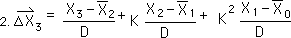
To see what a double unfurling means let us look at the 3rd Data Point of the First Directional. Below is the unfurling of this point.
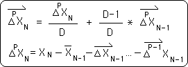
Below we separate the ∆X's into their constituent parts.
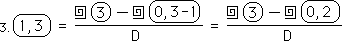
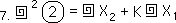
We now write the same directional in circle terms from Equation 18 above.
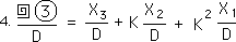
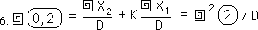
The single Unfurling of the 3rd Data Point gives us this equation.
Setting Equations 2 & 3 above equal to each other. Then we subtract out like elements from Equation 4 above. This gives us the equation below. Comparing Equations 16 & 18 we see that a single unfurling of the Decaying Average is the same as the Double Unfurling of the Raw Data divided by D, Hence the last term of the equation.
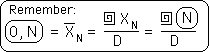
We remember the general definition for the Decaying Average from Equation 10 in the General Proof. This is the Fractal Root Pattern.
We substitute the Unfurling expressions for the Decaying Averages of Equation 5.
Multiplying through by D, we get the following expression. This is what we would expect with the nested function, an unfurling of a furled function. So once again our unfurling expression behaves predictably.
Below is the general expression for the double unfurling of Raw Data. This is nothing surprising. It is only the application of the function upon itself.
Below we convert to circle notation.
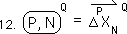
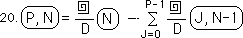
Again because the P factor is unchanged in an unfurling, this expression for a double unfurling also applies to the General Directional. Its expression is listed below.
Finally because the Unfurling Function is a function, no matter how many times it is applied to furl up the data, in this case Q times, the first time it is used to unfurl the Data it will only lower the Unfurling exponent by 1, Q-1 in the example below, and will Unfurl the Directionals to their first point, as is directed by the function. Below is the most general expression for the multiple Unfurling Function.
So now we have an idea what a multiple unfurling is. Soon we will examine its spatial manifestation. But for now we will move on to the Unraveling Function.
We introduced the concept of taking the Decaying Average to the second power, squaring the circle function. We promised that we would discuss what this means. Below are the parallel terms from Equations 16 & 21 in the general proof.
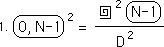
We write it below as an N instead of an N-1.
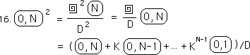
We remember the furled definition for the Decaying Average, the Fractal Root Pattern
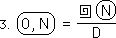
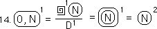
Let us write it with exponents. In some ways the circle around the Decaying Average, (0,N), is a function of the raw data. The circle around the Decaying Average represents the Raw Data Unfurled once and divided by D.
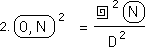
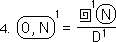
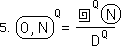
So if we take the circle of the Decaying Average to the second power it means that the Data is Unfurled twice and divided by D squared. Similarly employing the circle function over the Decaying Average Q times would mean to unfurl the Data Q times and divide by D to the Qth power. This is shown below.
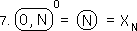
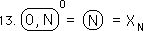
Let us employ this equation when Q = 0.
We see that the Decaying Average to the zeroth power is equal to the Raw Data itself.
We remember from the Derivative Notebook that the Raw Data is also equal to the zeroth level in the Change Series.
We set the Decaying Average to the zeroth power equal to the zeroth level in the Change Series below.
We replace the zero by a P in the appropriate places and find that the zeroth power of the general directional is equal to the general element of the Change Series. This is shown in the equation below. We have not demonstrated this logical connection yet but will find that it is a consistent link in the developments to come.
We now use the arrow as a function indicator similar to the circle function. When it is to the zeroth power in the equation below, it doesn't exist as in the equation above.
When the circle is the first power then we have the standard directional series, which are averages of averages.
When we raise the directional to the Qth power, it represents the Qth level of Averages. We will get a better idea what this means in the discussions to come.
Let us return to our zeroth power Decaying Average, which equals the raw Data. (Equation 7 above.)
The first power the Decaying Average equals the Raw Data unfurled divided by D. (Equation 4 above.) Unfurling divided by D equals the Circle Function, the Unraveling function. So we ravel the Data with another circle.
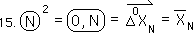
Hence the Data to the second power is the Decaying Average. This result is very important in converting the Directionals to functions of the Raw Data and vice versa.
The Decaying Average to the 2nd power is unfurled singly below in terms of Decaying Average rather than a double unfurling with the raw Data.
The general directional to the second power unfurls the same way as the zeroth directional because only the N part of the Directional is affected by unfurling. The single unfurling of the general Directional is shown below. This result is very important to the derivation that follows.
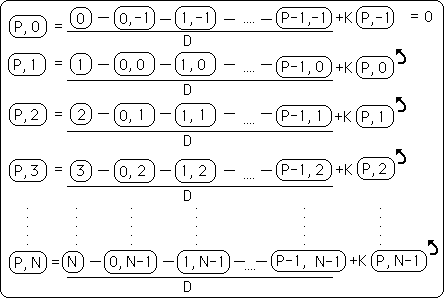
Below are the definitional equations for the general directionals.
Below are extensions of the general Directionals in terms of the general equations listed above with the circle notation.
The Pth Directional at the zeroth point always equals zero. The Pth Directional at the first point equals the first point subtracted from all the prior Directionals divided by D. All the prior Directionals, in this first case only, equal zero. Therefore the first point of all the Directionals is always equal to the first Data Point divided by D. Both of these results are consistent with prior results. {See Deviation Notebook.}
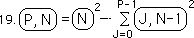
Lining up the like Directionals, i.e., Directionals with the same P, we find that we can rewrite the general Directional as the following equation, based upon Equation 17 above. Basically we are furling and raveling our directionals simultaneously.
Below is the rewrite of the above equation with a summation.
We reduce the equation from its second power to its first power by unraveling it once, as per definition.